Coupling principle

Acyclic Dependencies Principle

The ADP deals with the relationships between components, the tension between developability & logical design.

WHAT: What really is ADP?

Principle: Component dependence graphs do not have any accepted circles. Imagine in a graph, you are standing at any component, follow the dependent arrow, if you can return to the correct component, it means your graph violates.

Allow no cycles in the component dependency graph.

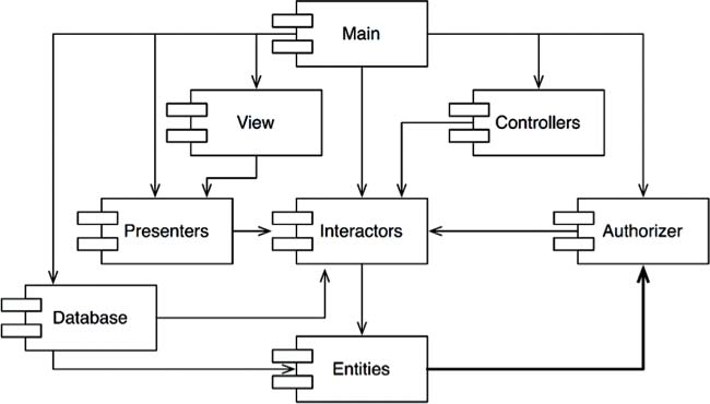
For example, in the following graph, we can easily go from the Authorizer component, through Interactors, to Entities and then back to it.

WHY

The goal of this principle is to avoid the situation of "Morning after syndrome" - you come home late and commit your code, but someone else comes home later, trying to fix their code. cause your code to stop running.

And an important cause of this situation is cross-dependency between components in the system. The problem will become more complicated and occur more frequently if a source code is shared with a larger team. By applying this principle we can avoid such situations.

HOW: “Dependency Inversion Principle” (The D in SOLID principles)

Ta có thể sử dụng nguyên lý này để đảo chiều phụ thuộc. VD: Trong hình mối quan hệ giữa Entities & Authorizer. Muốn bỏ phụ thuộc Entities lên Authorizer, tách interface mà Entities dùng từ Authorizer ra thành 1 component mới cả Entities & và Authorizer đều phụ thuộc lên, VD: Permission.

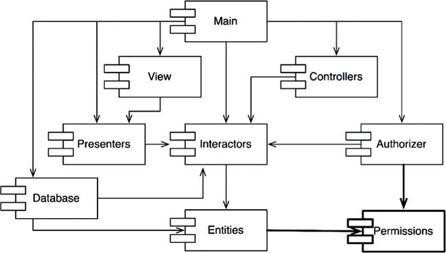
We can use this principle to reverse dependence. For example: In the picture the relationship between Entities & Authorizer. If you want to remove Entities dependency on Authorizer, separate the interface that Entities use from Authorizer into a new component that both Entities & Authorizer depend on, eg: Permission.

Top-down design

The issues we have discussed so far lead to an inescapable conclusion: The component structure cannot be designed from the top down. It is not one of the first things about the system that is designed, but rather evolves as the system grows and changes.

Some readers may find this point to be counterintuitive. We have come to expect that large-grained decompositions, like components, will also be high-level functional decompositions.

When we see a large-grained grouping such as a component dependency structure, we believe that the components ought to somehow represent the functions of the system. Yet this does not seem to be an attribute of component dependency diagrams.

In fact, component dependency diagrams have very little do to with describing the function of the application. Instead, they are a map to the buildability and maintainability of the application. This is why they aren’t designed at the beginning of the project. There is no software to build or maintain, so there is no need for a build and maintenance map. But as more and more modules accumulate in the early stages of implementation and design, there is a growing need to manage the dependencies so that the project can be developed without the “morning after syndrome.” Moreover, we want to keep changes as localized as possible, so we start paying attention to the SRP and CCP and collocate classes that are likely to change together.

One of the overriding concerns with this dependency structure is the isolation of volatility. We don’t want components that change frequently and for capricious reasons to affect components that otherwise ought to be stable. For example, we don’t want cosmetic changes to the GUI to have an impact on our business rules.

We don’t want the addition or modification of reports to have an impact on our highest-level policies. Consequently, the component dependency graph is created and molded by architects to protect stable high-value components from volatile components.

As the application continues to grow, we start to become concerned about creating reusable elements. At this point, the CRP begins to influence the composition of the components. Finally, as cycles appear, the ADP is applied and the component dependency graph jitters and grows.

If we tried to design the component dependency structure before we designed any classes, we would likely fail rather badly. We would not know much about common closure, we would be unaware of any reusable elements, and we would almost certainly create components that produced dependency cycles. Thus the component dependency structure grows and evolves with the logical design of the system.

Stable Dependencies Principle

Definition

A module should only depend upon modules that are more stable than it is.

Some components are designed to be volatile. We expect them to change. Any of these should not depend on a component that is difficult to change. We should depend in the direction of stability. Again employing the DIP can help us to apply this principle breaking dependency on a stable component.

Stability

What is meant by “stability”? Stand a penny on its side. Is it stable in that position? You would likely say “no.” However, unless disturbed, it will remain in that position for a very long time. Thus stability has nothing directly to do with frequency of change. The penny is not changing, but it is difficult to think of it as stable.

Webster’s Dictionary says that something is stable if it is “not easily moved.” Stability is related to the amount of work required to make a change. On the one hand, the standing penny is not stable because it requires very little work to topple it. On the other hand, a table is very stable because it takes a considerable amount of effort to turn it over. How does this relate to software? Many factors may make a software component hard to change—for example, its size, complexity, and clarity, among other characteristics. We will ignore all those factors and focus on something different here. One sure way to make a software component difficult to change, is to make lots of other software components depend on it. A component with lots of incoming dependencies is very stable because it requires a great deal of work to reconcile any changes with all the dependent components. \

The diagram in Figure 14.5 shows X, which is a stable component. Three components depend on X, so it has three good reasons not to change. We say that X is responsible to those three components. Conversely, X depends on nothing, so it has no external influence to make it change. We say it is independent.

Figure 14.6 shows Y, which is a very unstable component. No other components depend on Y, so we say that it is irresponsible. Y also has three components that it depends on, so changes may come from three external sources. We say that Y is dependent.

Stability Metric

How can we measure the stability of a component? One way is to count the number of dependencies that enter and leave that component. These counts will allow us to calculate the positional stability of the component.

• Fan-in: Incoming dependencies. This metric identifies the number of classes outside this component that depend on classes within the component.

• Fan-out: Outgoing depenencies. This metric identifies the number of classes inside this component that depend on classes outside the component.

• I: Instability: I = Fan-out , (Fan-in + Fan-out). This metric has the range [0, 1]. I = 0 indicates a maximally stable component. I = 1 indicates a maximally unstable component.

The Fan-in and Fan-out metrics are calculated by counting the number of classes outside the component in question that have dependencies with the classes inside the component in question. Consider the example in Figure 14.7.

Let’s say we want to calculate the stability of the component Cc. We find that there are three classes outside Cc that depend on classes in Cc. Thus, Fan-in = 3. Moreover, there is one class outside Cc that classes in Cc depend on. Thus, Fan- out = 1 and I = 1/4.

In C++, these dependencies are typically represented by #include statements. Indeed, the I metric is easiest to calculate when you have organized your source code such that there is one class in each source file. In Java, the I metric can be calculated by counting import statements and qualified names.

When the I metric is equal to 1, it means that no other component depends on this component (Fan-in = 0), and this component depends on other components (Fan-out > 0). This situation is as unstable as a component can get; it is irresponsible and dependent. Its lack of dependents gives the component no reason not to change, and the components that it depends on may give it ample reason to change.

In contrast, when the I metric is equal to 0, it means that the component is depended on by other components (Fan-in > 0), but does not itself depend on any other components (Fan-out = 0). Such a component is responsible and independent. It is as stable as it can get. Its dependents make it hard to change the component, and its has no dependencies that might force it to change.

The SDP says that the I metric of a component should be larger than the I metrics of the components that it depends on. That is, I metrics should decrease in the direction of dependency.

How does it work?

The instability of a module is defined as the ratio between the number if incoming dependencies and the number of combined incoming/outgoing dependencies.

Instability = # incoming dependencies / (# incoming dependencies + # outgoing dependencies)

An stable module is harder to change than an instable module, because it has more modules that need to be checked and changed.

An instable module needs to change more often than an stable module, because it has more modules that it depends on.

If you build a dependency hierarchy that keeps the most stable modules on the top, and the most instable modules on the bottom, the system will be easier to change and maintain.

Not all componeny should be stable

If all the components in a system were maximally stable, the system would be unchangeable. This is not a desirable situation. Indeed, we want to design our component structure so that some components are unstable and some are stable.

The diagram in Figure 14.8 shows an ideal configuration for a system with three components. The changeable components are on top and depend on the stable component at the bottom. Putting the unstable components at the top of the diagram is a useful convention because any arrow that points up is violating the SDP (and, as we shall see later, the ADP).

The diagram in Figure 14.9 shows how the SDP can be violated.

Flexible is a component that we have designed to be easy to change. We want Flexible to be unstable. However, some developer, working in the component named Stable, has hung a dependency on Flexible. This violates the SDP because the I metric for Stable is much smaller than the I metric for Flexible. As a result, Flexible will no longer be easy to change. A change to Flexible will force us to deal with Stable and all its dependents.

To fix this problem, we somehow have to break the dependence of Stable on Flexible. Why does this dependency exist? Let’s assume that there is a class C within Flexible that another class U within Stable needs to use (Figure 14.10).

We can fix this by employing the DIP. We create an interface class called US and put it in a component named UServer. We make sure that this interface declares

all the methods that U needs to use. We then make C implement this interface as shown in Figure 14.11. This breaks the dependency of Stable on Flexible, and forces both components to depend on UServer. UServer is very stable (I = 0), and Flexible retains its necessary instability (I = 1). All the dependencies now flow in the direction of decreasing I.

Abstract Components

You may find it strange that we would create a component—in this example, UService—that contains nothing but an interface. Such a component contains no executable code! It turns out, however, that this is a very common, and necessary, tactic when using statically typed languages like Java and C#. These abstract components are very stable and, therefore, are ideal targets for less stable components to depend on.

When using dynamically typed languages like Ruby and Python, these abstract components don’t exist at all, nor do the dependencies that would have targeted them. Dependency structures in these languages are much simpler because dependency inversion does not require either the declaration or the inheritance of interfaces.

Stable Abstraction Principle

Introduce

The Stable Abstractions Principle (SAP) sets up a relationship between stability and abstractness. On the one hand, it says that a stable component should also be abstract so that its stability does not prevent it from being extended. On the other hand, it says that an unstable component should be concrete since it its instability allows the concrete code within it to be easily changed. Thus, if a component is to be stable, it should consist of interfaces and abstract classes so that it can be extended. Stable components that are extensible are flexible and do not overly constrain the architecture. The SAP and the SDP combined amount to the DIP for components. This is true because the SDP says that dependencies should run in the direction of stability, and the SAP says that stability implies abstraction. Thus dependencies run in the direction of abstraction.

The DIP, however, is a principle that deals with classes—and with classes there are no shades of gray. Either a class is abstract or it is not. The combination of the SDP and the SAP deals with components, and allows that a component can be partially abstract and partially stable.

Measuring Abstraction

The A metric is a measure of the abstractness of a component. Its value is simply the ratio of interfaces and abstract classes in a component to the total number of classes in the component.

• Nc: The number of classes in the component.

• Na: The number of abstract classes and interfaces in the component.

• A: Abstractness. A = Na ÷ Nc.

The A metric ranges from 0 to 1. A value of 0 implies that the component has no abstract classes at all. A value of 1 implies that the component contains nothing but abstract classes.

The main sequence

We are now in a position to define the relationship between stability (I) and abstractness (A). To do so, we create a graph with A on the vertical axis and I on the horizontal axis (Figure 14.12). If we plot the two “good” kinds of components on this graph, we will find the components that are maximally stable and abstract at the upper left at (0, 1). The components that are maximally unstable and concrete are at the lower right at (1, 0).

Not all components fall into one of these two positions, because components often have degrees of abstraction and stability. For example, it is very common for one abstract class to derive from another abstract class. The derivative is an abstraction that has a dependency. Thus, though it is maximally abstract, it will not be maximally stable. Its dependency will decrease its stability.

Since we cannot enforce a rule that all components sit at either (0, 1) or (1, 0), we must assume that there is a locus of points on the A/I graph that defines reasonable positions for components. We can infer what that locus is by finding the areas where components should not be—in other words, by determining the zones of exclusion

The Zone of Pain

Consider a component in the area of (0, 0). This is a highly stable and concrete component. Such a component is not desirable because it is rigid. It cannot be extended because it is not abstract, and it is very difficult to change because of its stability. Thus we do not normally expect to see well-designed components sitting near (0, 0). The area around (0, 0) is a zone of exclusion called the Zone of Pain.

Some software entities do, in fact, fall within the Zone of Pain. An example would be a database schema. Database schemas are notoriously volatile, extremely concrete, and highly depended on. This is one reason why the interface between OO applications and databases is so difficult to manage, and why schema updates are generally painful.

Another example of software that sits near the area of (0, 0) is a concrete utility library. Although such a library has an I metric of 1, it may actually be nonvolatile. Consider the String component, for example. Even though all the classes within it are concrete, it is so commonly used that changing it would create chaos. Therefore String is nonvolatile.

Nonvolatile components are harmless in the (0, 0) zone since they are not likely to be changed. For that reason, it is only volatile software components that are problematic in the Zone of Pain. The more volatile a component in the Zone of Pain, the more “painful” it is. Indeed, we might consider volatility to be a third axis of the graph. With this understanding, Figure 14.13 shows only the most painful plane, where volatility = 1.

The Zone of Uselessness

Consider a component near (1, 1). This location is undesirable because it is maximally abstract, yet has no dependents. Such components are useless. Thus this area is called the Zone of Uselessness.

The software entities that inhabit this region are a kind of detritus. They are often leftover abstract classes that no one ever implemented. We find them in systems from time to time, sitting in the code base, unused.

A component that has a position deep within the Zone of Uselessness must contain a significant fraction of such entities. Clearly, the presence of such useless entities is undesirable.

Avoiding the zone of exclusion

It seems clear that our most volatile components should be kept as far from both zones of exclusion as possible. The locus of points that are maximally distant from each zone is the line that connects (1, 0) and (0, 1). I call this line the Main Sequence.

A component that sits on the Main Sequence is not “too abstract” for its stability, nor is it “too unstable” for its abstractness. It is neither useless nor particularly painful. It is depended on to the extent that it is abstract, and it depends on others to the extent that it is concrete.

The most desirable position for a component is at one of the two endpoints of the Main Sequence. Good architects strive to position the majority of their components at those endpoints. However, in my experience, some small fraction of the components in a large system are neither perfectly abstract nor perfectly stable. Those components have the best characteristics if they are on, or close, to the Main Sequence.

Distance from the main sequence

This leads us to our last metric. If it is desirable for components to be on, or close, to the Main Sequence, then we can create a metric that measures how far away a component is from this ideal.

• D3 : Distance. D = |A+I–1| . The range of this metric is [0, 1]. A value of 0 indicates that the component is directly on the Main Sequence. A value of 1 indicates that the component is as far away as possible from the Main Sequence.

Given this metric, a design can be analyzed for its overall conformance to the Main Sequence. The D metric for each component can be calculated. Any component that has a D value that is not near zero can be reexamined and restructured.

Statistical analysis of a design is also possible. We can calculate the mean and variance of all the D metrics for the components within a design. We would expect a conforming design to have a mean and variance that are close to zero. The variance can be used to establish “control limits” so as to identify components that are “exceptional” in comparison to all the others.

In the scatterplot in Figure 14.14, we see that the bulk of the components lie along the Main Sequence, but some of them are more than one standard deviation (Z = 1) away from the mean. These aberrant components are worth examining more closely. For some reason, they are either very abstract with few dependents or very concrete with many dependents.

Another way to use the metrics is to plot the D metric of each component over time. The graph in Figure 14.15 is a mock-up of such a plot. You can see that some strange dependencies have been creeping into the Payroll component over the last few releases. The plot shows a control threshold at D = 0.1. The R2.1 point has exceeded this control limit, so it would be worth our while to find out why this component is so far from the main sequence.